Topographic indices from DEM¶

This is a short demo of the pysoilmap.features module - which allows deriving some simple topographic features.

Setup¶

[1]:

import ee
import matplotlib.pyplot as plt
import numpy as np

[2]:

import pysoilmap.ee as psee
from pysoilmap.features import Topography, diff_gauss
from pysoilmap.plotting import add_colorbar

We will download a DEM via the Google Earth Engine API. For this, you will have to authenticate with a google account here:

[3]:

psee.initialize()

The SRTM data is in WGS84 (degree). We want a coordinate system in meters to get meaningful units in derived quantities.

So let’s request the data in 3-degree Gauss-Kruger zone 3, and pick a Region around Tübingen:

[4]:

crs = 'epsg:31467'
xmid = 3_499_159
ymid = 5_371_552
xscale = yscale = 90
xdim = 100
ydim = 100
xmin = xmid - xdim / 2 * xscale
xmax = xmid + xdim / 2 * xscale
ymin = ymid - ydim / 2 * yscale
ymax = ymid + ydim / 2 * yscale

The transform defines how pixel coordinates are calculated from the matrix indices. We have to set a negative yscale and set the offset to ymax in order to have the (0, 0) pixel as the top left corner:

[5]:

# [xScale, xShearing, xTranslation, yShearing, yScale, yTranslation]
transform = [xscale, 0, xmin, 0, -yscale, ymax]

Now download DEM from SRTM 30m dataset:

[6]:

srtm = ee.Image("USGS/SRTMGL1_003")
dem = psee.download_image(
    srtm,
    'elevation',
    crs=crs,
    transform=transform,
    xdim=xdim,
    ydim=ydim,
)

In order to download bigger images (>= 50 MB) you would have to export them to your google drive first, and then manually download from there. The export can be started as follows:

[7]:

if False:
    task = ee.batch.Export.image.toDrive(srtm, **{
        'description': 'DEM',
        'crs': crs,
        'dimensions': [xdim, ydim],
        'crsTransform': transform,
    })
    task.start()
    task.status()

Define a function for plotting multiple variables at once:

[8]:

def plot_maps(*images, **kwargs):
    extent = np.array([0, xmax - xmin, 0, ymax - ymin]) / 1000
    rows = len(images)
    cols = len(images[0])
    fig, axes = plt.subplots(
        rows, cols,
        squeeze=False,
        figsize=(cols * 3, rows * 3))
    for i, row in enumerate(images):
        for j, (title, image) in enumerate(row.items()):
            ax = axes[i, j]
            ax.set_title(title)
            ax.imshow(image, extent=extent, **kwargs)
            add_colorbar(ax, size=0.1, pad=0.07)
            if i == rows - 1:
                ax.set_xlabel('x [km]')
            if j == 0:
                ax.set_ylabel('y [km]')
    plt.tight_layout()

[9]:

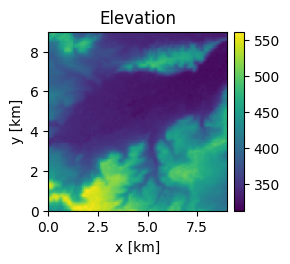
plot_maps({'Elevation': dem})

Features¶

By default Topography calculates spatial derivatives using central differencing:

[10]:

topo_0 = Topography(
    dem,
    cellsize=(xscale, yscale),
    crs=crs,
    transform=transform,
)

Alternatively, spatial derivatives can be calculated using a Gaussian derivative filter. This corresponds to smoothing the DEM with a Gaussian filter, and then calculating the derivative. It can be understood as calculating the derivative at a given lengthscale:

[11]:

topo_2 = Topography(
    dem,
    cellsize=(xscale, yscale),
    crs=crs,
    transform=transform,
    diff=diff_gauss,
    sigma=2,
)

[12]:

topo_5 = Topography(
    dem,
    cellsize=(xscale, yscale),
    crs=crs,
    transform=transform,
    diff=diff_gauss,
    sigma=5,
)

[13]:

topos = [topo_0, topo_2, topo_5]

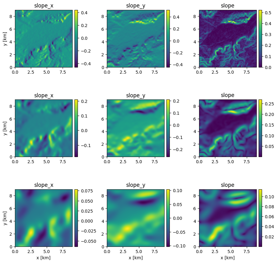
Slope (tangent)¶

[14]:

plot_maps(*[{
    "slope_x": topo.slope_x(),
    "slope_y": topo.slope_y(),
    "slope": topo.slope(),
} for topo in topos])

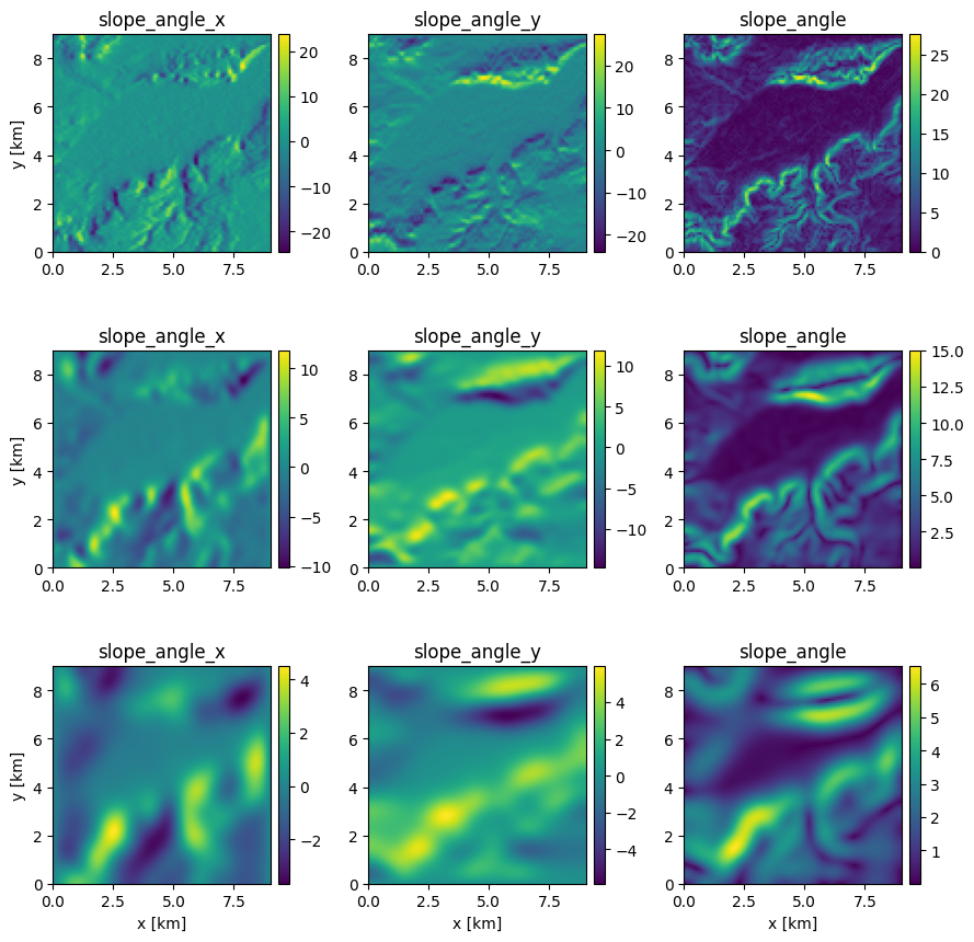
Slope (angle)¶

[15]:

plot_maps(*[{
    "slope_angle_x": topo.slope_angle_x() * 180 / np.pi,
    "slope_angle_y": topo.slope_angle_y() * 180 / np.pi,
    "slope_angle": topo.slope_angle() * 180 / np.pi,
} for topo in topos])

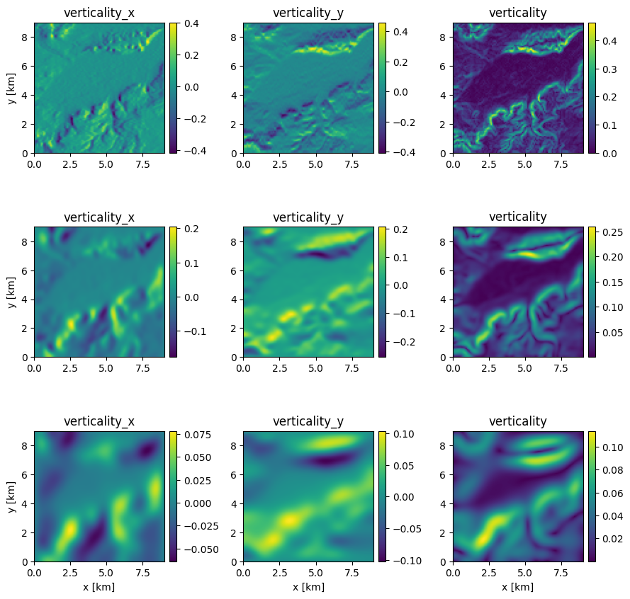
Slope (sine)¶

[16]:

plot_maps(*[{
    "verticality_x": topo.verticality_x(),
    "verticality_y": topo.verticality_y(),
    "verticality": topo.verticality(),
} for topo in topos])

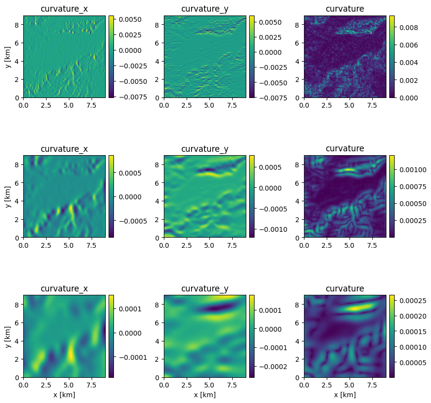
Curvature¶

[17]:

plot_maps(*[{
    "curvature_x": topo.curvature_x(),
    "curvature_y": topo.curvature_y(),
    "curvature": topo.curvature(),
} for topo in topos])

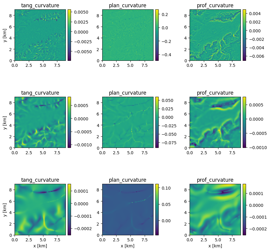
[18]:

plot_maps(*[{
    "tang_curvature": topo.tang_curvature(),
    "plan_curvature": topo.plan_curvature(),
    "prof_curvature": topo.prof_curvature(),
} for topo in topos])

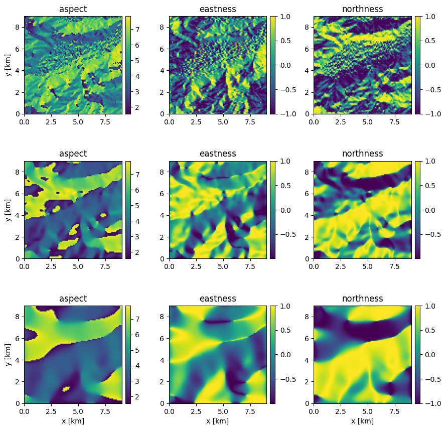
Aspect¶

[19]:

plot_maps(*[{
    "aspect": topo.aspect(),
    "eastness": topo.eastness(),
    "northness": topo.northness(),
} for topo in topos])

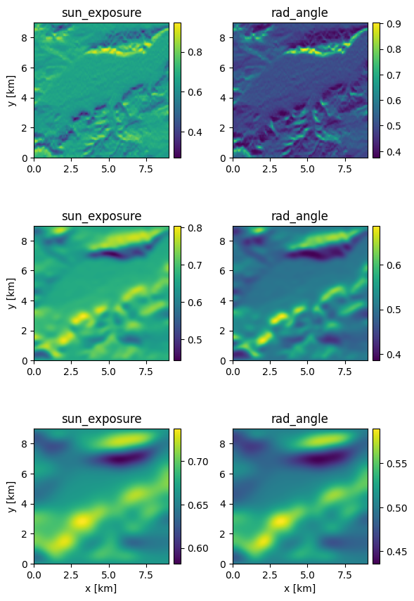
Irradiation¶

[20]:

plot_maps(*[{
    "sun_exposure": topo.sun_exposure(),
    "rad_angle": topo.rad_angle(),
} for topo in topos])

When downloading bigger images, it may be necessary to load them in chunks. This can be done as follows:

[21]:

dem23 = psee.download_image(
    srtm,
    'elevation',
    crs=crs,
    transform=transform,
    xdim=xdim,
    ydim=ydim,
    xtile=2,
    ytile=3,
    threads=3,
)
assert (dem23 == dem).all()